Introduction
A new regulation from the National Highway Traffic Safety Administration (FMVSS 141) has been enacted that requires all electric vehicles meet certain sound output requirements when operating in different scenarios. This is due to concerns that the low sound output of many electric vehicles can make them hazardous to pedestrians. The regulation provides target sound pressure levels over the frequency range for a number of different operating conditions of the vehicles (stationary, reverse, forward motion, etc.).
The goal of this was project was to design a method for testing the compliance of electric vehicles (EVs) using readily available audio equipment. Traditional methods for conducting acoustic tests of these kind often require expensive hardware far outside the price range of consumers and some researchers. In addition, proprietary software is often required to implement the acoustic analysis (1/3 octave band analysis) specified in this kind of acoustic test. Python scripts were developed to offer an alternative process with comparable results, although with a greater margin of error due to limitations of calibration.
The code developed here is open source. Check it out on Github.
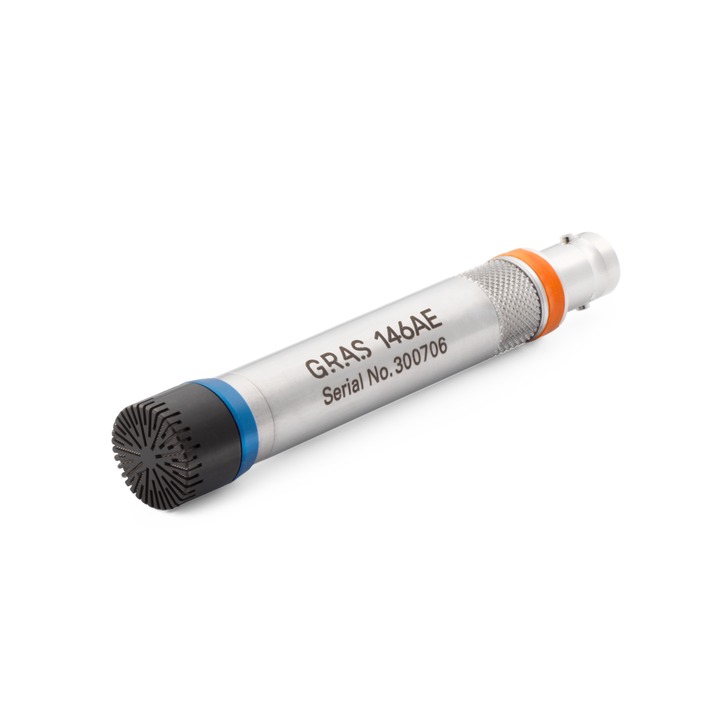
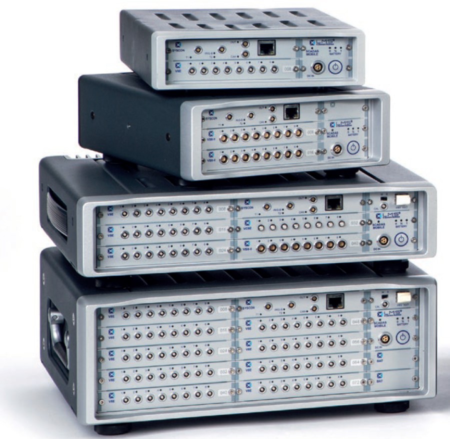
From left to right: GRAS free-field reference microphone, Siemens LMS SCADAS Recorders, and Siemens PLM Software.
Equipment
The basic signal chain for collecting acoustic measurements involves first, a reference microphone with a flat frequency response, a linear microphone preamplifier, an analog to digital converter, and finally appropriate software that allows for the calibration and analysis of the measured data. For this project any consumer grade audio equipment available will work. In our case, we used the equipment shown below for measurement and calibration. This equipment is available for just over $200, but also requires a laptop and software to record audio samples. Any DAW or simple audio software will suffice. In our testing we use Adobe Audition. Audacity or REAPER would be good free of cheap alternatives.
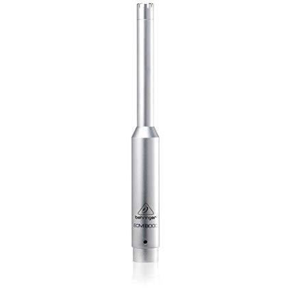
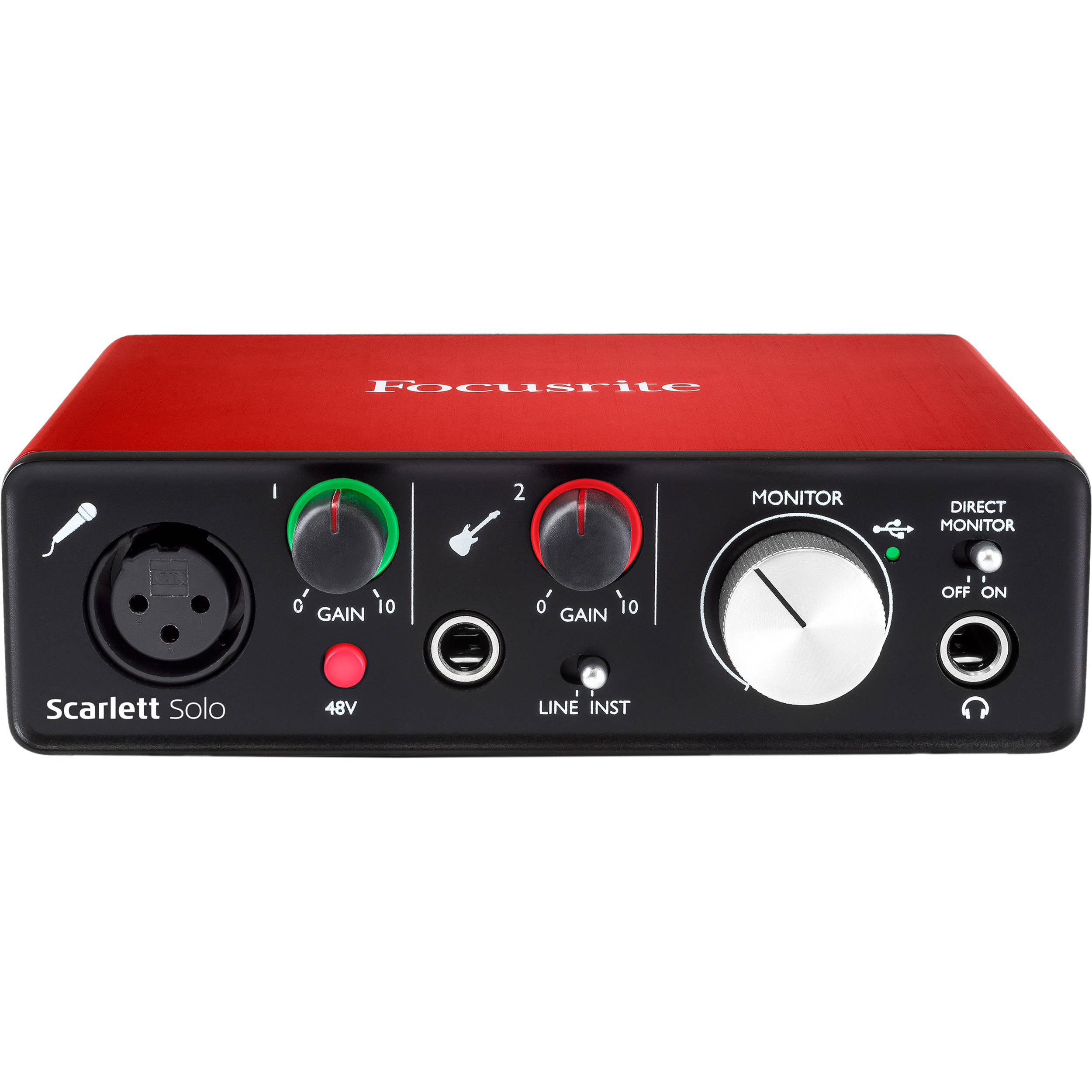
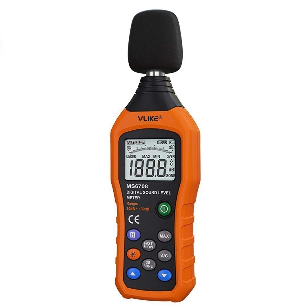
From left to right: Behringer ECM8000 ($58.99) , Focusrite Scarlett Solo ($100.95), and the VLIKE Sound Level Meter ($55.99)
Setup and Calibration
The standard specifies exactly how the test for each case should be carried out. For example there are different testing procedures for the vehicle while stationary, in reverse, moving at 10 km/hr, 20 km/hr, and 30 km/hr. Please refer to the standard for full details. Before any testing can begin the measurement system must be calibrated as follows. Note the file naming conventions. These must be followed so the accompanying Python scripts can operate correctly.
Play a consistent sound (e.g. 1 kHz tone) that is well above the ambient noise level.
Use a calibrated A weighted dB SPL meter to measure the level at the same location as the microphone.
Note this value and use it in the name of the calibration file. (
cal_74_04-21-2019.wavfor 74 dB SPL)Record about 5-10 seconds of the noise signal via the reference microphone.
Ensure that the recorded signal is not too high nor too low. Adjust the preamp gain if needed.
Turn off the signal.
Record about 5-10 seconds of the ambient sound in the testing environment. (
amb_04-21-2019.wav)Finally conduct each test recording with at least 2 seconds of audio. (
stat_04-21-2019_1.wav)
The final number of the test file indicates which run of that kind of test the audio recording corresponds to. This allows the user to provide and plot multiple runs of the same kind of test in the same directory. Use the proper filename format for each testing type for proper plotting following the guide below.
| Test type | Filename example |
| Stationary | stat_04-21-2019_1.wav |
| Reverse | rev_04-21-2019_1.wav |
| 10 km/hr | 10_04-21-2019_1.wav |
| 20 km/hr | 20_04-21-2019_1.wav |
| 30 km/hr | 30_04-21-2019_1.wav |
| Ambient | amb_04-21-2019.wav |
| Calibration | cal_74_04-21-2019.wav |
Store all test files in a single directory and install and run the code as shown below to create plots for each of the test cases. Note the provided directory must contain a calibration and ambient audio file in order to produce any kind of plot. The number of test files in a single directory can be arbitrary as long as a number (run index) is provided for each test file, as explained above.

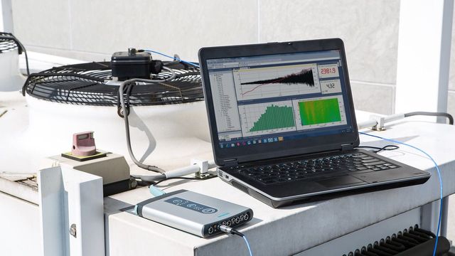
An example testing setting showing the microphone, the audio interface, and laptop for recording audio samples.
Data Analysis
Once tests have been run and recordings are available, the Python scripts (available on GitHub) can be used to provide an analysis of the data. Follow the instructions on README to get the code setup and running. In order to analyze the data a number of steps are performed within the scripts.
First, all of the audio files provided are loaded as floating point data. The ambient and calibration files are identified by their file names, as are the rest of the test files. Each test file must be calibrated before any data is analyzed. To perform this calibration a calibration factor is determined, which allows for translation from dBFS to dB SPL. Using the calibration recording, an A weighting filter is applied and an FFT is used to determine the energy in each frequency bin. Different block sizes are used to replicate different response times of SPL meters (fast vs. slow). Finally the energy in each of the bins is summed, which represents the total signal energy and is the same energy measured by the SPL meter. This is used along with recorded level to calibrate individual test recordings.
Each test recording is parsed to extract the relevant test details and the A weighting filter is applied as well. The calibration factor is used to convert the measurements in dBFS to dBA SPL and the signal is then split in to 1/3 octave bands for analysis against the provided spec. The spec provides a minimum dBA SPL level for a number of ANSI 1/3 octave bands, shown on the plot below. Plots for each sample are automatically generated that show the content both in the time domain as well as the frequency domain, along with the 1/3 octave band requirements for easy comparison.

An example of a single plot that is provided as output from the developed scripts. This plot shows the analyzed signal in the time domain as well as the SPL level over 13 ANSI 1/3 octave bands for comparison against the FMVSS 141 specified minimums.
Resources
The algorithm for computing 1/3 octave bands came from this whitepaper by Microstar Laboratories.
Additional details on 1/3 octave analysis can be found in this very detailed NI reference manual.
Special thanks to endolith for the A weighting filter implementation.